"/home/yossef/notes/personal/ml/linear_regression.md"

path: personal/ml/linear_regression.md

- **fileName**: linear_regression
- **Created on**: 2025-04-30 02:43:06

Linear regression is a statistical method used to model the relationship
between a dependent variable and one or more independent variables

so it's making a model by represented relation between some variable or
characteristic for agent so making a connection and found a pattern to make
a relation between this and making prediction based on this relation.

linear regression is type of supervised learning (learning from labeled data)
mapping this datasets to points with the most optimized linear function

Example:

if we want to predict house price we consider various factor such as house age,
distance from the main road, location, area and number of room,
linear regression uses all these parameter to predict house price as it consider
a linear relation between all these features and price of house.

it's worked based on the best fit line

best fit line: the error between the predict point and the actual value
should be minimum, so it's represent a relation between variables to line

Here Y is called a dependent or target variable and X is called an
independent variable also known as the predictor of Y. There are many
types of functions or modules that can be used for regression. A linear
function is the simplest type of function. Here, X may be a single feature
or multiple features representing the problem.

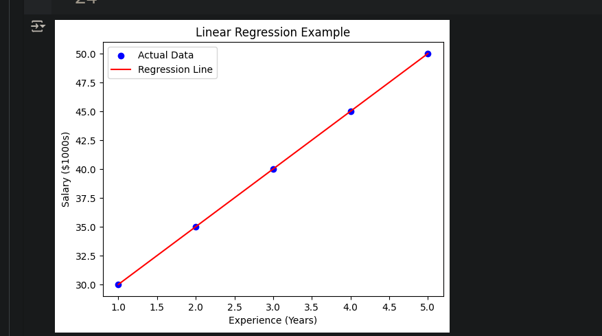
Example: Predicting Salary Based on Experience

Data:
Experience (Years) (X) Salary ($1000s) (Y)

You can see there's a linear relationship:
as experience increases, salary increases.

Linear Regression Goal:

We want to find a line (function) that best predicts salary (Y) given years
of experience (X).

The line has the form:

Where:
m = slope (how much Y changes when X increases)
b = intercept (the value of Y when X = 0)

tensorflow exmaple:

import numpy as np
from sklearn.linear_model import LinearRegression
import matplotlib.pyplot as plt

# Data
X = np.array([1, 2, 3, 4, 5]).reshape(-1, 1)  # Years of experience
y = np.array([30, 35, 40, 45, 50])  # Salary in $1000s

# Train the model
model = LinearRegression()
model.fit(X, y)

# Predict
predictions = model.predict(X)

# Plot
plt.scatter(X, y, color='blue', label='Actual Data')
plt.plot(X, predictions, color='red', label='Regression Line')
plt.xlabel('Experience (Years)')
plt.ylabel('Salary ($1000s)')
plt.title('Linear Regression Example')
plt.legend()
plt.show()

some conditions to get accurate results

• Linearity: must there is a relation between the dependent and independent
• Independence: this mean that the value of dependent value don't depend
  on any thing
• Homoscedasticity: remains constant across all values of the
  independent variable (X)-> (check down if not understand ;))
• Normality: residuals(points) should follow a bell-shaped curve

Case 1: Homoscedasticity

the errors are small and stay roughly the same → Model is valid.

Case 2: Heteroscedasticity

The error increases as experience increases → Model is not reliable.

2. Multiple Linear Regression

Multiple linear regression involves more than one independent variable and one dependent variable. The equation for multiple linear regression is:

Where:

• ( y) is the dependent variable
• ( X1, X2, ...., Xn ) are the independent variables
• ( B0 ) is the intercept
• ( B1, B2, ...., Bn) are the slopes (coefficients) of the respective independent variables

No Multicollinearity (in Multiple Linear Regression)

Definition:
There should be little or no correlation between
independent variables in a multiple linear regression model.

Why it matters:

If two or more independent variables are highly
correlated (i.e., they provide overlapping information), the
model can't accurately determine which variable is actually
affecting the dependent variable.

What is Multicollinearity?

• Multicollinearity means X₁ and X₂ are very similar.
• This causes confusion for the model.
• The model may overestimate or underestimate
  coefficients, leading to unreliable predictions.

Example:

Suppose you’re trying to predict house prices based on:

• X₁: size in square feet
• X₂: number of rooms

But usually, bigger houses have more rooms — so X₁ and
X₂ are highly correlated.

As a result:

• The model can't decide whether size or rooms is more
  important.
• Coefficients become unstable.

Problem:

If there's multicollinearity, multiple linear regression
becomes inaccurate and less interpretable.

Tip for Detecting Multicollinearity:

• Use a correlation matrix or Variance Inflation Factor
  (VIF).
• If VIF > 5 or VIF > 10 → this is a strong
  multicollinearity warning!

Additivity (in Multiple Linear Regression)

Definition:
The model assumes that the effect of changes in a predictor variable
on the response variable is consistent regardless of the values of
the other variables. This assumption implies that there is no
interaction between variables in their effects on the dependent
variable.

Why it matters:

If this assumption is violated (i.e., there are interactions
between variables), the model will not be able to account for the
combined effects properly, leading to inaccurate predictions and
interpretations.

Example:

Suppose we are predicting house prices using two variables:

• X₁: size in square feet
• X₂: number of rooms

The assumption of additivity implies that the effect of increasing
the size (X₁) on the price will be the same regardless of how many
rooms (X₂) the house has.

Feature Selection in Multiple Linear Regression

Feature selection is the process of choosing the most relevant
predictor variables to include in the model. This helps to:

• Improve model accuracy
• Prevent overfitting
• Enhance interpretability

Selecting the best features ensures that the model doesn't use
irrelevant or redundant predictors that might introduce noise and
increase variance.

Overfitting: Overfitting occurs when the model fits the training data too closely,

Real-World Applications of Multiple Linear Regression (MLR)

Real Estate Pricing

is used to predict property prices based on
multiple factors such as:

• Location
• Size
• Number of bedrooms

Financial Forecasting

to predict stock prices or economic
indicators based on multiple influencing factors, including:

• Interest rates
• Inflation rates
• Market trends

Agricultural Yield Prediction

Farmers can apply MLR to estimate crop yields using variables
like:

• Rainfall
• Temperature
• Soil quality
• Fertilizer usage

E-commerce Sales Analysis

An e-commerce company can use MLR to analyze how various factors
impact sales, such as:

• Product price
• Marketing promotions
• Seasonal trends

for cost function for linear regression

./cost_function_linear_regression.md

Gradient Descent for Linear Regression

A linear regression model can be trained using the optimization
algorithm gradient descent. This method iteratively updates
the model’s parameters to reduce the Mean Squared Error (MSE)
on a training dataset.

Goal: Minimize the Cost Function

The goal is to minimize the cost function (typically the MSE),
which results in a best-fit line for the data. To do this,
we update the parameters ( theta_1 ) and ( \theta_2 )
to reduce the Root Mean Squared Error (RMSE).

We start with random initial values for ( \theta_1 ) and
( \theta_2 ), then update them iteratively using the gradient
descent algorithm:

Where:

• ( \alpha ) is the learning rate
• ( J ) is the cost function
• ( \theta_j ) represents the parameters being optimized

Iterative Updates

Each update step moves ( \theta_1 ) and ( \theta_2 ) slightly
closer to the values that minimize the cost function.

Over many iterations, gradient descent converges toward the
optimal parameters for the best linear regression line.

example using pytorch:

import torch
import torch.nn as nn
import matplotlib.pyplot as plt
import numpy as np
from sklearn.metrics import confusion_matrix, ConfusionMatrixDisplay

# 1. Generate synthetic data
# Experience (in years)
X = torch.tensor([[1.0], [2.0], [3.0], [4.0], [5.0]])
# Salary in thousands
Y = torch.tensor([[30.0], [35.0], [40.0], [45.0], [50.0]])

# 2. Define a simple linear regression model
class LinearRegressionModel(nn.Module):
    def __init__(self):
        super().__init__()
        self.linear = nn.Linear(1, 1)  # input and output are both 1D

    def forward(self, x):
        return self.linear(x)

model = LinearRegressionModel()

# 3. Loss function: Mean Squared Error
criterion = nn.MSELoss()

# 4. Optimizer: Gradient Descent (SGD)
optimizer = torch.optim.SGD(model.parameters(), lr=0.01)

# 5. Training the model
epochs = 200
loss_values = []

for epoch in range(epochs):
    model.train()
    
    # Forward pass: compute predicted y
    y_pred = model(X)

    # Compute loss
    loss = criterion(y_pred, Y)
    loss_values.append(loss.item())

    # Zero gradients, backward pass, update weights
    optimizer.zero_grad()
    loss.backward()
    optimizer.step()

    # Plot every 50 epochs
    if epoch % 50 == 0:
        plt.figure()
        plt.scatter(X.numpy(), Y.numpy(), color='blue', label='Actual')
        plt.plot(X.numpy(), y_pred.detach().numpy(), color='red', label='Predicted')
        plt.title(f'Epoch {epoch} | Loss: {loss.item():.2f}')
        plt.xlabel('Experience (Years)')
        plt.ylabel('Salary (Thousands)')
        plt.legend()
        plt.grid(True)
        plt.show()

# 6. Final prediction
final_pred = model(X).detach().numpy()

# 7. Confusion Matrix (only for demonstration)
# Convert to discrete bins to simulate classification
actual_classes = (Y // 5).numpy().flatten().astype(int)
predicted_classes = (torch.tensor(final_pred) // 5).numpy().flatten().astype(int)

# Compute and show confusion matrix
cm = confusion_matrix(actual_classes, predicted_classes)
disp = ConfusionMatrixDisplay(confusion_matrix=cm)
disp.plot()
plt.title("Confusion Matrix (Binned Salaries)")
plt.show()

# 8. Plot loss over epochs
plt.figure()
plt.plot(loss_values)
plt.title("Loss over Epochs")
plt.xlabel("Epoch")
plt.ylabel("MSE Loss")
plt.grid(True)
plt.show()

references

• tensorflow

• geekforgeeks

• text

• notebook

  continue:./cost_function_linear_regression.md
  before:./knn.md